2. RDE - Robox Development Environment

2.1. First step

In order to getting started with the controller, we need a memory card where we have to copy RTE and some configuration files. A new memory card will have the folder KEY that contain Robox licence and the folder /f@ with the last version of RTE. The RTE binary file can also be downloaded from Robox website.

Note

Don’t delete the folder KEY from the memory card. I contain the licence.

After the installation of RDE, RCE and Icmap, we need to copy in the installation directory, usually Robox, the license in order to compile programs. The license is provided by Robox.

Note

Microsoft c++ redistributable 2010 and 2015 x86 must be installed on your computer

Note

RDE is the IDE of Robox, RCE is R3 and OB compiler, ICmap is the AGV’s maps compiler. ICmap can be installed only if we use AGV, otherwise is not needed.

RDE main windows

2.2. New RTE project

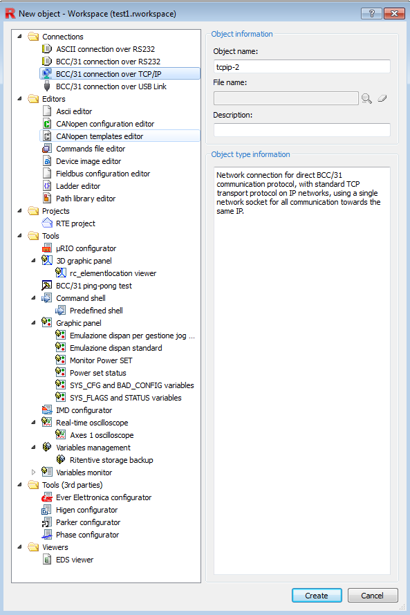
RDE like others IDEs (Eclipse, Atom, Visual studio code, etc.) use workspaces. One workspace may contain more than one project. So before creating a new RTE project, a workspace have to be created.

In the menu bar, the workspace menu, allow to open, create and manage workspaces, also to access the predefined examples. We can create as many workspaces as we want. Usually one project or machine program have its own workspace.

The New RDE workspace and RTE project animation illustrate step by step how:

• Create a new space
• Create a connection to a controller
• Create a new project
• Choose the compiler

New RDE workspace and RTE project

RTE project was created, and a connection. The connection should have the same ip address of the controller.

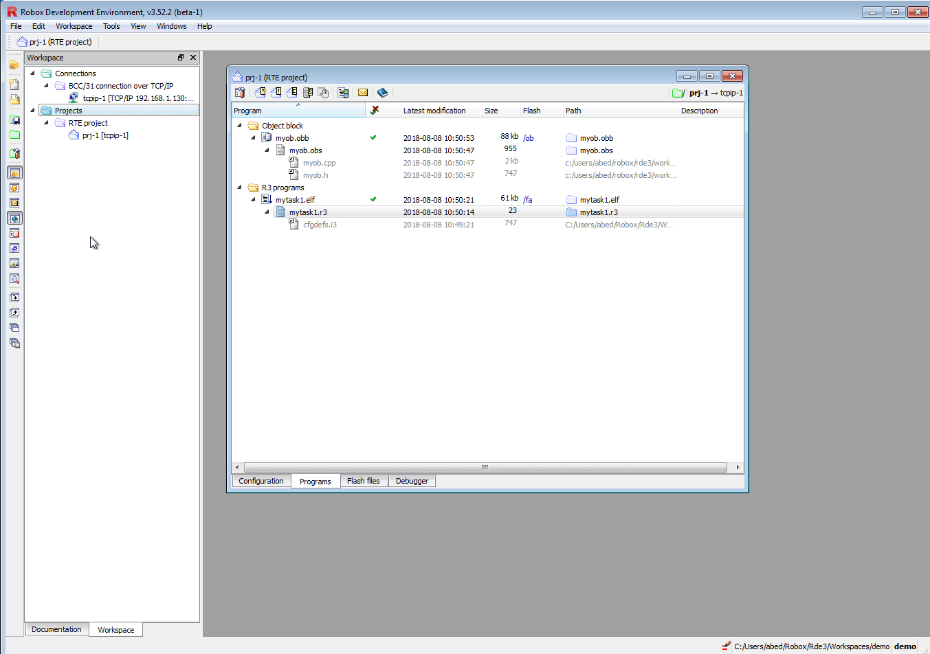
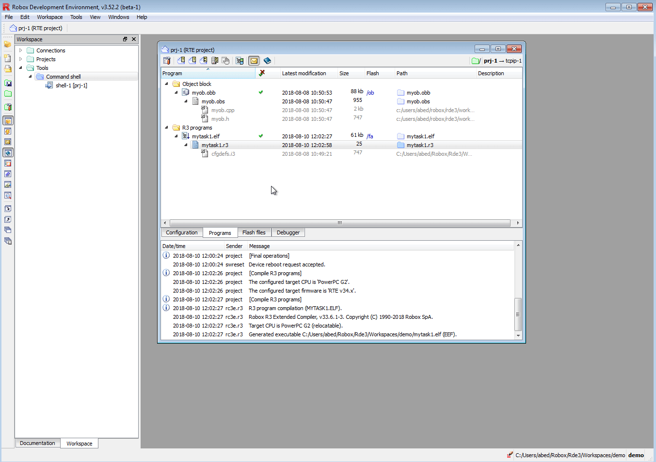
The following animation illustrate how a R3 program and an Object block can be created in an RTE project.

R3 program and Object block (OB)

Note

Remember to save the workspace after any modification: Workspace –> Save workspace

Tasks and Rules are R3 programs. When the keyword $TASK n where n is the task number, e.g. $TASK 1, the R3 program become a task. If the keyword $rule is used the R3 program become a RULE.

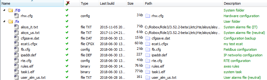
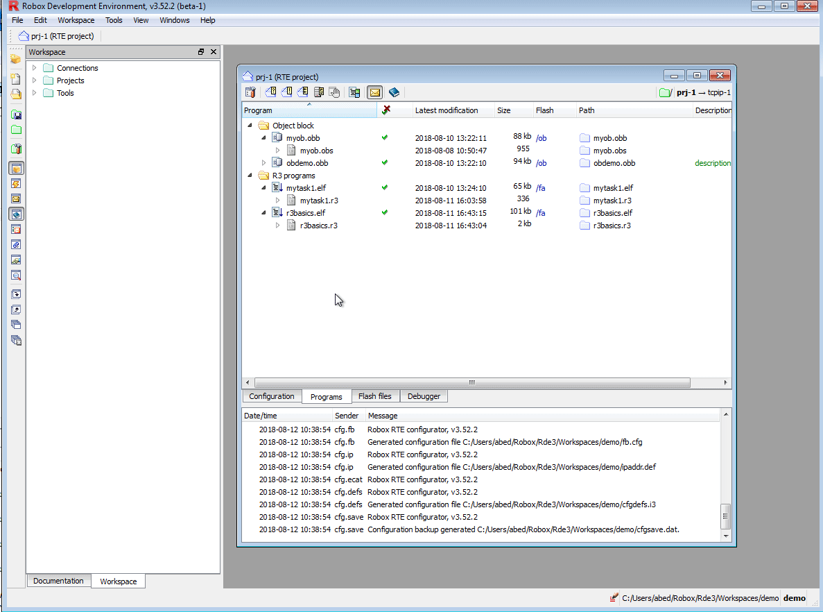
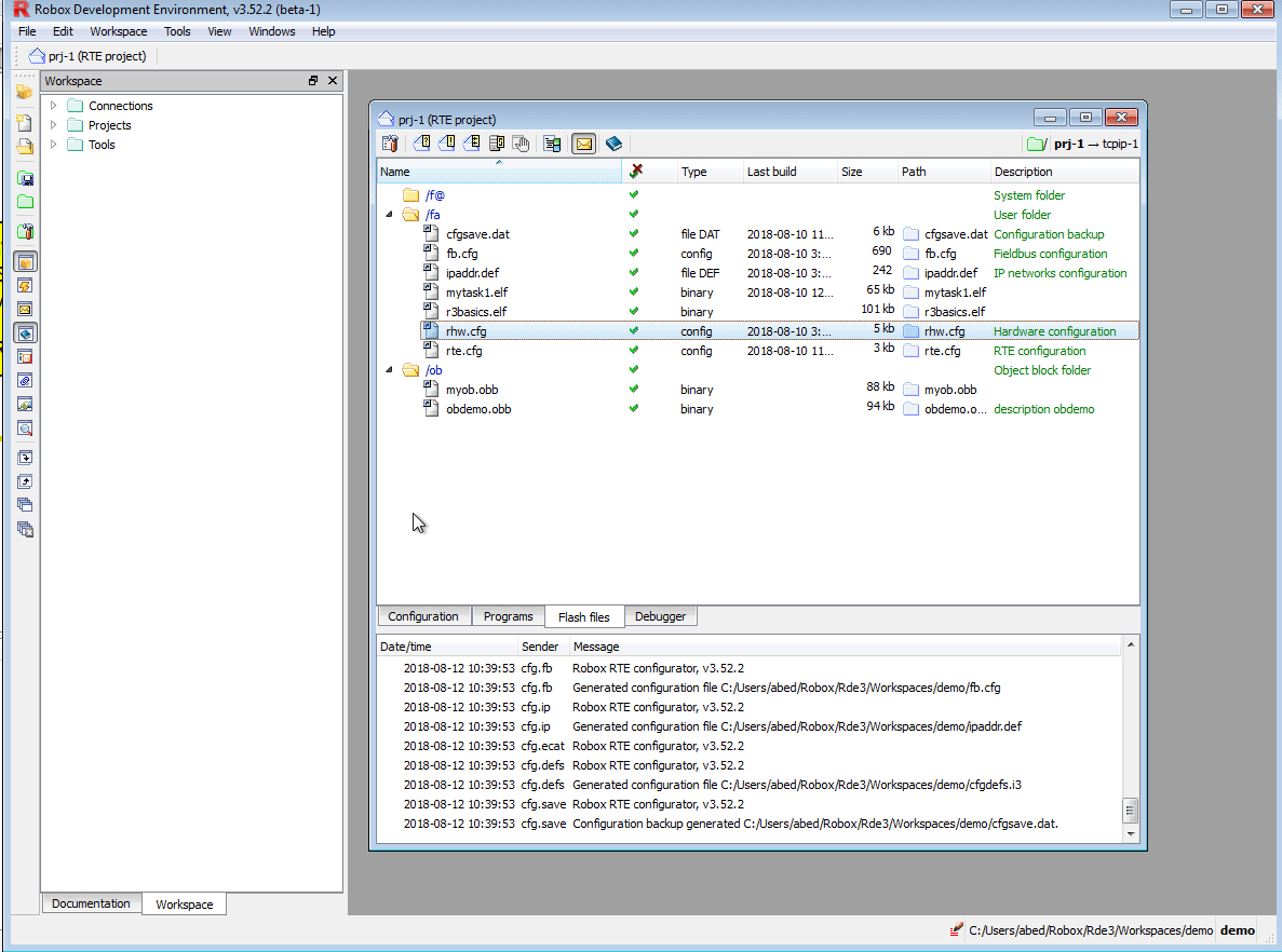
An RTE system files can have different folders. This demo use the default folders:

• f@ : RTE binary file
• fa : R3 programs and configuration files
• ob : Oject block compiled files

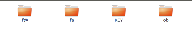
Memory card default folders

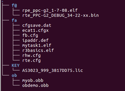
Memory card default folders tree

Note

An RTE project can have until eight R3 programs as TASKS and one R3 program as RULE. This doesn’t mean we have one rule.

Demo used in this chapter

2.3. RDE basics

2.3.1. Flash image

After the creation of a new project, the memory card should be prepared with the right folders and files, Memory card default folders tree. The RTE binary file can be downloaded from Robox website. Project files and programs can be created from RDE.

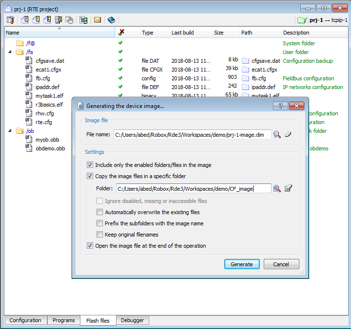
Mainly it is enough to have on the memory card the hardware configuration file and the ip address file, in order to connect to the controller from RDE. Anyway, when a new project is created is more conveniente to create the project image from RDE and copy them to the memory card.

Connect the memory card to your computer using a flash card reader if using RP1 or a microSd card reader if using RP2. And copy the generated folders (the image) to the memory card following the procedure showed in the animation.

The following animation show the procedure to prepare the first project image.

First setup

Prepare the flash card the first time

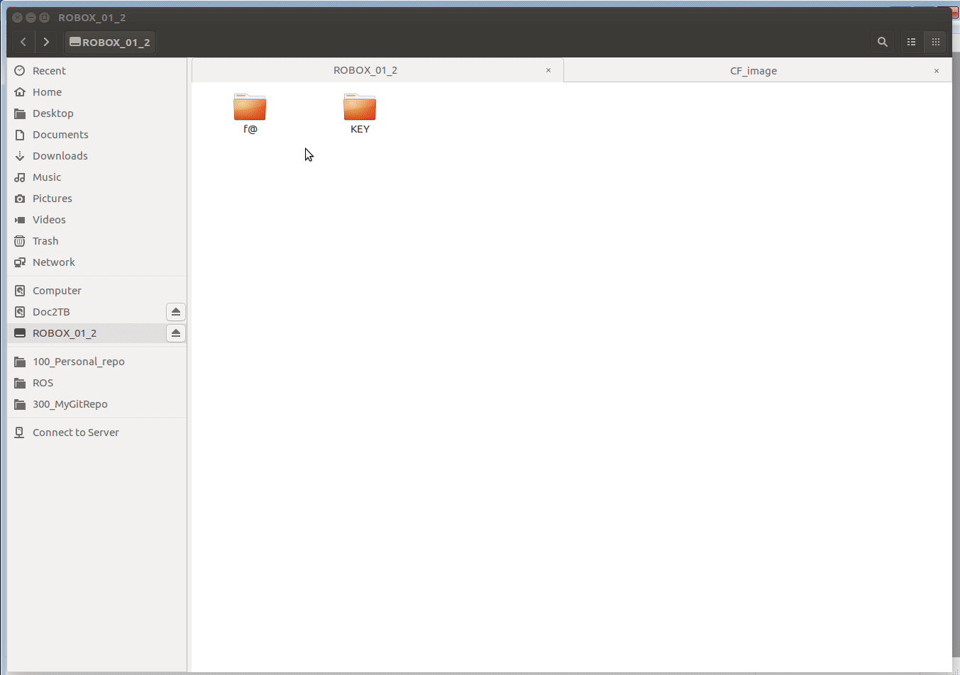
The image is generated in any folder that you want, but it is better to create a folder in the working workspace called CF_image and generate the image files in it. When the image files are generated, they will be copied into the memory card.

Flash image files

Note

Don’t copy the or replace the /f@ folder. The f@ should contain the necessary files.

When the memory card contains all the necessary files and folders, any modification to the project can be downloaded to the controller directly from RDE, and the controller is ready to communicate with RDE. Plug the ethernet cable on the second ethernet port of e.g. RP1.

2.3.2. Tools

We already see how to create a new project, create a connection to the controller, and copy the main files and folders to the memory card. In order to see if the controller can communicate with the computer we can use the windows command ping or linux command nmap.

Our goal is to use RDE, so we will see how to use RDE tools in order to connect to the controller. RDE have different tools: console (like linux terminal or windows prompt), oscillosope, graphic panels, etc.

The scope of this section is to show how to use tools to monitor variables. Don’t care now about R3 syntax, even if the code should be clear if you know another programming language. Keep in mind that we will monitor some variables which value is changing.

Connect the controller to the computer via an ehternet cable, turn it on (give power) and be sure that your computer have the same ip class address. If the controller have e.g. 192.168.1.130 ip address the computer should have 192.168.1.xxx where xxx is a number different from the ip address of the controller, in this case 130.

2.3.2.1. Console

The following animation show how we can create a console, connect it to the controller and use some commands.

Notice that the connection name is the project, not the connection to controller. It is conveniente to connect the project to controller connection, and all other tools to the project.

create a console

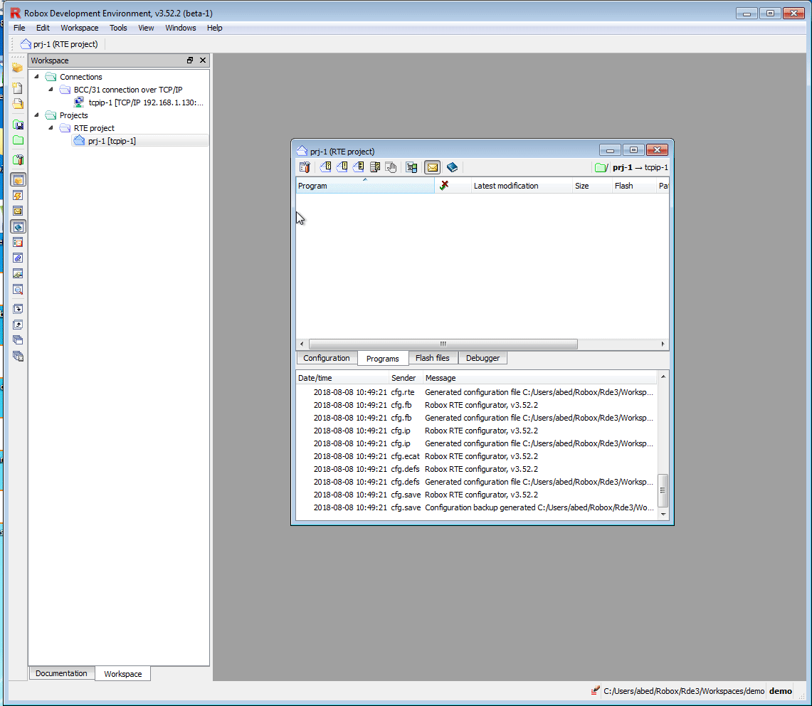
The project can be compiled and download to the controller, using the button Make project or Rebuild project. You can select wich folders you want to download to the controller. Usually we download the mofied folders.

Note

Don’t select f@ folder when building the project.

Custom console commands can be created using Robox X-script language.

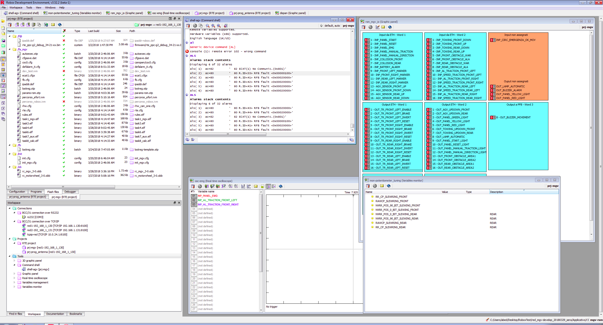
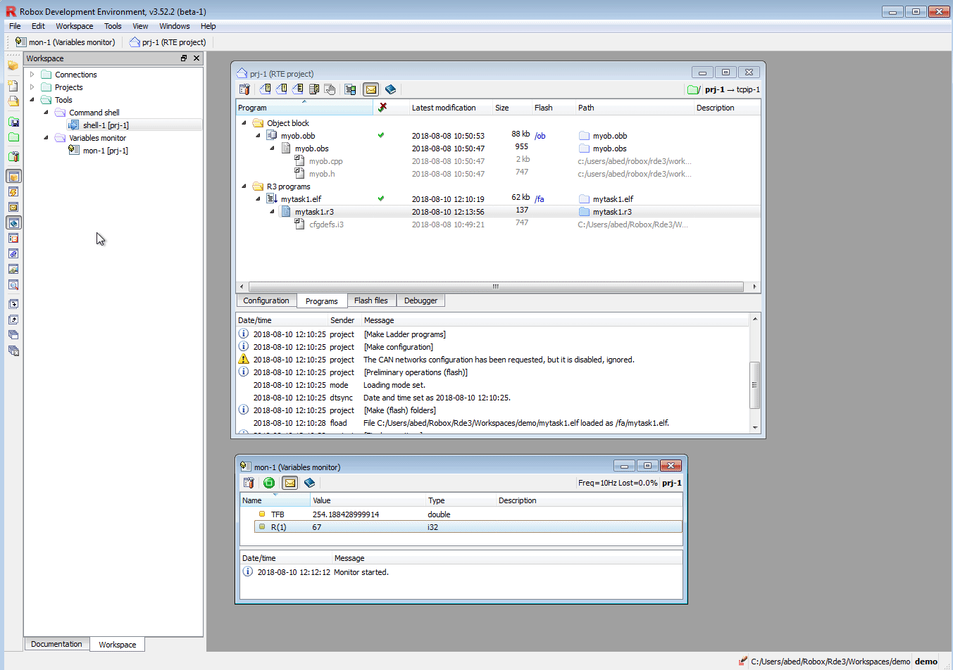
2.3.2.2. Variable monitor

In the following animation we will modify the R3 program in order to create a one second timer, then build and download the project to the controller. We will create also a variable monitor to show the value of the timer variable.

Modify program and download to controller. Create a variable monitor.

2.3.2.3. Graphic panel

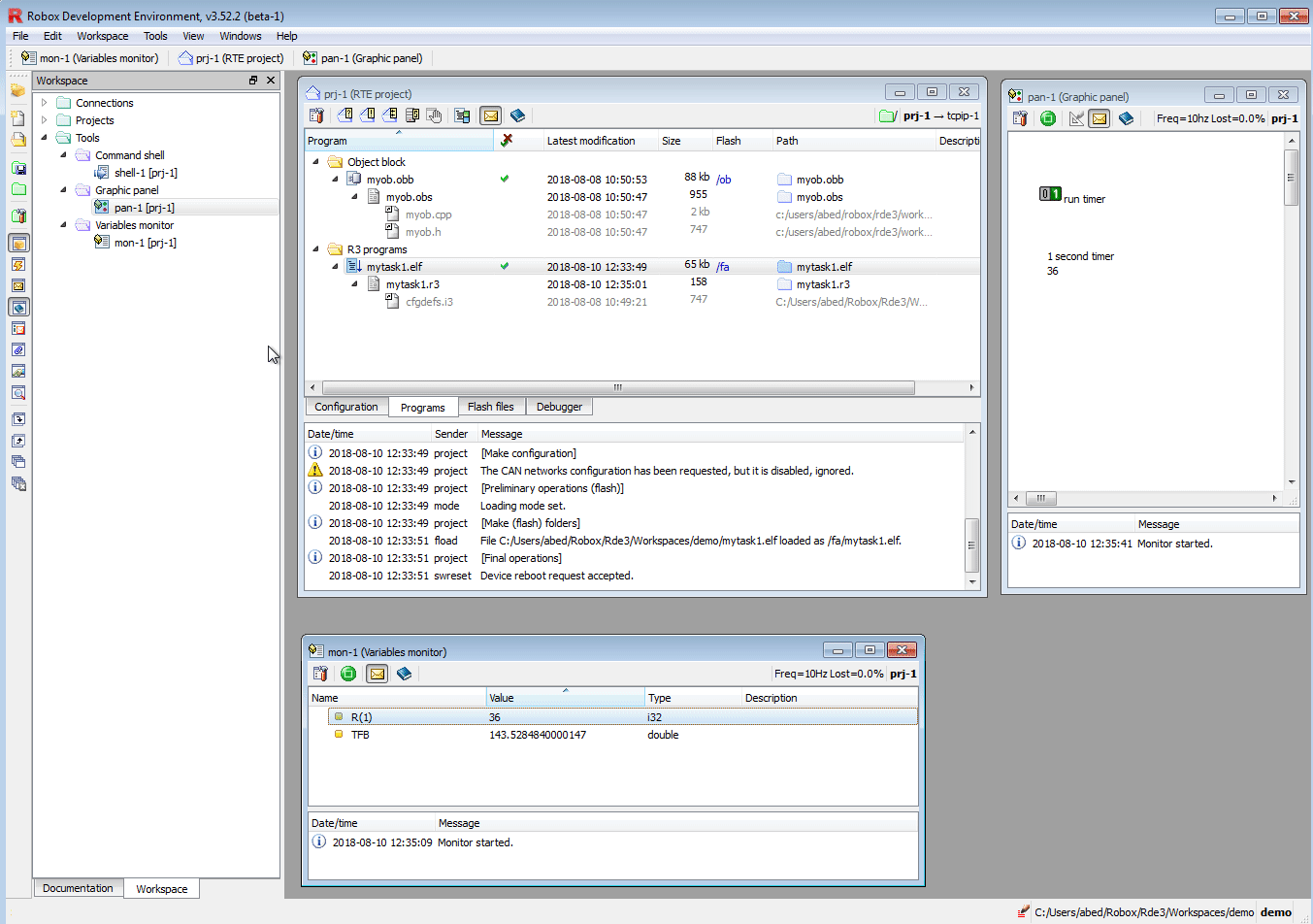
The next modification we will create a graphic panel with one button and one textbox. The button will be related to a variable or register to stop or run the timer. The textbox is used to show the value of the timer.

graphic panel

Create a graphic panel (HMI)

2.3.2.4. Oscilloscope

In order to illustare the use of an oscilloscope we modify the R3 program in order to generate a sinusoidal wave.

Oscilloscope

Create a sinusoidal wave and monitor it in an oscillosope.

2.3.2.5. 3D graphic panel

Create a 3D graphic panel, where we will show a box that move along the y axis in an alternate motion.

3D graphic panel

3D graphic panels can be cutomized using X-script language, see X-script chapter for more informations.

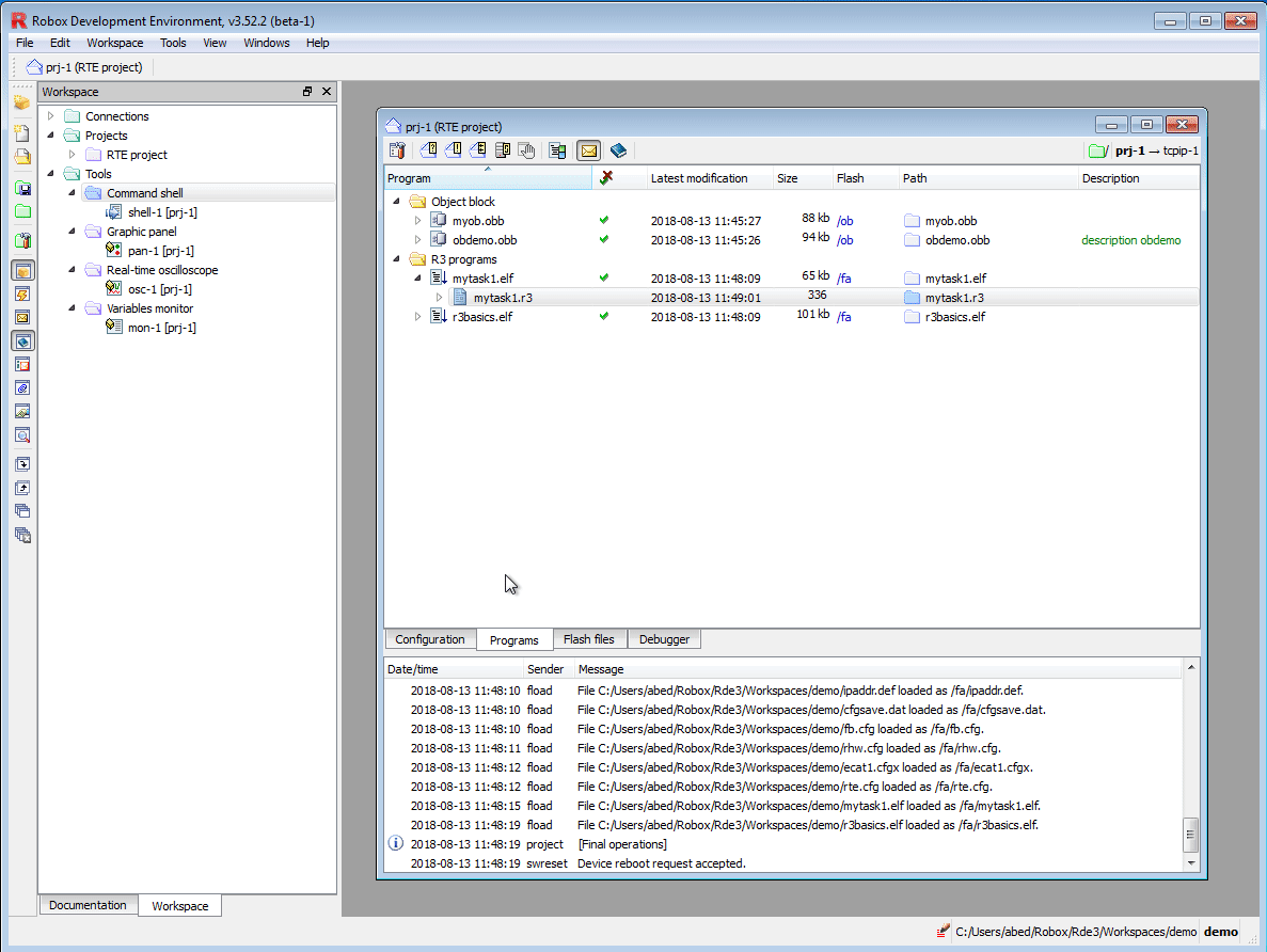
2.4. Important folders and files

In the memory card are present a lot of files and folders. Some of them are important to know what they are, others no. In the documentation of RDE you can find an explanation of those files.

Files in flash. Auto generated files

RDE will generate automaticcaly files in the default folders. So for now don’t care too much about them. First confidence with the use of RDE should be gained, then advanced concepts will be invetigated.

2.5. Tools

From the workspace we can access the tools provided by RDE. Different kinds of tools are provided to debug and monitor the software: panels, oscilloscope, variable monitors and command shell, etc. Some of them we have already see.

Objects available in a workspace

Some predefined objects are already created by Robox e.g. axis powerset graphic panel.

In the following image we can see some tool created and present in the workspace. We can notice that this workspace have two projects.

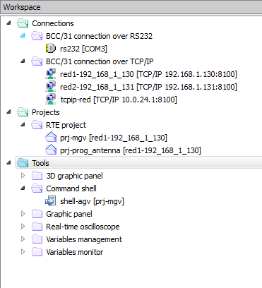
Some tools in the workspace

2.5.1. Connections

In order to connect a project or a tool to a controller, we need to create a connection. If we connect to the controller via ethernet cable, as we already see previously, we need to create a tcp/ip connection with the ip address of the controller.

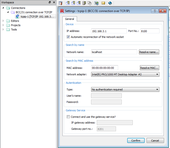
Tcp connection

If we connect to the controller via serial cable, we need to create a serial connection.

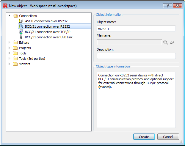
New object. Serial connection

2.5.2. Command shell

The shell allow to interact with the controller via shell commands and device commands. The most important commands for debugging are sysinfo to get information about the controller, als to get the list of alarms in the stack and mreport to get a report about the activities of the controller, the result is a log menu that can be exported to text file..

We can make shortcuts to the most used commands. Click the mouse right button and go to set quick commands in order to define shortcuts. A list of defined shortcuts is available from the function keys [F1-F12] and from the action menu accessible from the mouse right click.

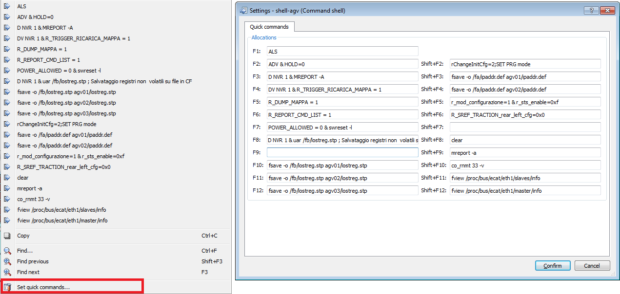
Command shell: Quick commands

There are different types of commands, some types to manage variables others to manage the flash card other the device. A list of commands is available in the official documentation.

We will see some of the most used commands divided by category. Several commands can be used alone or with options. More than one command can be sent together by using the \& operator. Take a look at Command shell: Quick commands in order to see the usage and syntax of some commands.

2.5.2.1. Variable management

• DV: Display variable value. The dv command allow us to monitor the value of variables e.g. dv nvr 1 display the value of the register nvr(1).
• SV: Set variable value
• FV: Force variable value
• RV: Release variable value

2.5.2.2. Device management

• adv Resets the device alarm
• sysinfo Get information on connected device.
• mreport It displays the events log. the option -a display all reports. Other options are available in order to filter the report.
• als It displays the contents of the alarms stack.
• swreset Request for software reset.
• uar Opens a file present in the flash card and refreshes the assignments to R, NVR, RR, NVRR, SR and NVSR with the current values but leaves the comment lines unchanged.

2.5.3. Flash management

• fsave Save file from flash.
• fview view a file from the flash.

2.5.4. Example of use

• nvr 1 5 Set the value of nvr register 1 to 5, equivalent to sv nvr 1 5
• nvr 4.2 1 Set the bit 2 of nvr register 4 to 1
• d inp_w 100
• d inp 1
• d nvr 1
• d nvr 2.3
• d nvr 1 5 Displays 5 registers starting from 1
• d nvr 1 5 -v Displays 5 registers starting from 1 with their index
• f_inp 300 Force logical state of input 300
• uar /fb/lostreg.stp Save the value of register in the file lostreg.stp

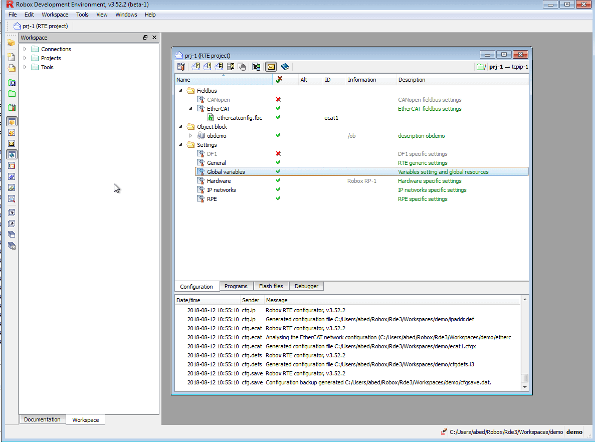
2.6. Bus configuration

Physical IO (Input-Ouput) are mapped into the memory of the controller, in the so called process image. IO are updated at the begining or the end of the periodic task (Rule). The cycle time is too short, about 5 ms, so it have no importance when it is update. So let’s suppose that the controller read the physical input pin_w at the begining of the periodic task and write the to the designated memory inp_w, and read of the output memory out_w and write to the physical output pout_w.

In the program the process image or logical IO are used, rarely physical IO are used in a program. IO memory area is an index area represented by 2 big arrays of words (16 bits), one for inputs inp_w and one for outputs out_w. In IEC 61131-3 these are represented as %IW and %QW. IO memory can be accessed also by single bit, using the 2 arrays inp(bit_index) and out(bit_index).

The indexes begin from 1 NOT from 0, e.g. input word 2 is inp_w(2) and the first bit of the word is inp_w(2).0 the correspond to inp(17).

2.6.1. Axioline

Robox controllers support natively Phoenix Axioline bus.

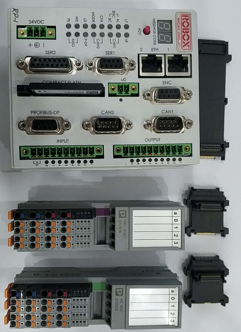
RP1 and Phoenix Axioline IO

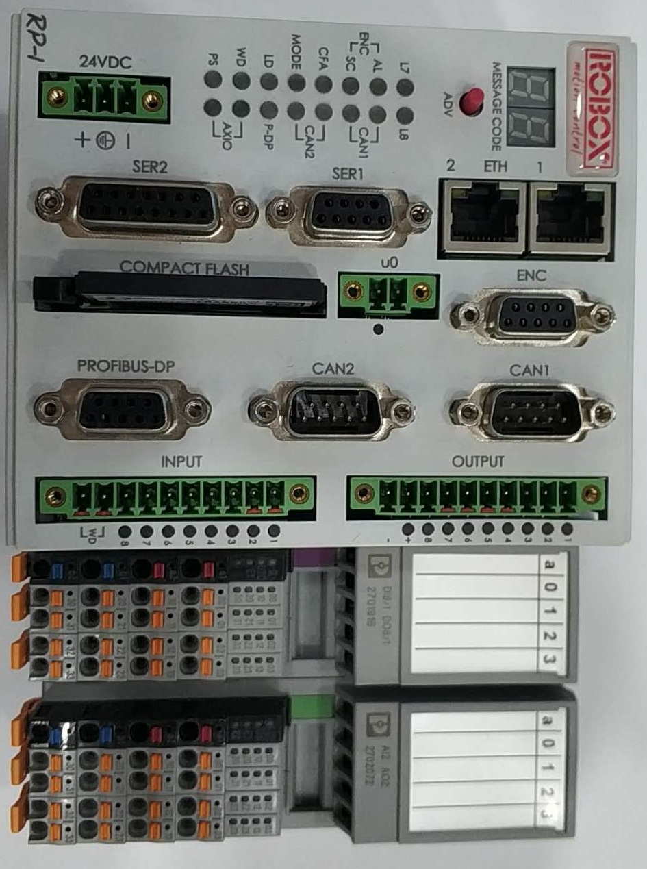
RP1 and Phoenix Axioline one digital IO module and one analog IO module

In the following animation we will add to the harware configuration one Phoenix Digital IO module (8 Digital inputs and 8 Digital outputs) and one analog module (2 analog inputs and 2 analog outputs) as shown in the previous pictures..

Axioline configuration. Add one Pheonix Digital IO module and one analog IO module

In the animation we choose automatic memory addressing, we can find the addresses in the flash file rhw.cfg :

IW 36 SLOT 3.01               ; AXL_F_DI8_1_DO8_1_1H (First 8 input group)
IW 37 SLOT 4.01               ; AXL_F_AI2_AO2_1H (Analog input channel 1)
IW 38 SLOT 4.02               ; AXL_F_AI2_AO2_1H (Analog input channel 2)

OW 36 SLOT 3.01               ; AXL_F_DI8_1_DO8_1_1H (First 8 output group)
OW 37 SLOT 4.01               ; AXL_F_AI2_AO2_1H (Analog output channel 1)
OW 38 SLOT 4.02               ; AXL_F_AI2_AO2_1H (Analog output channel 2)

The first physical input can be read on the address inp_w(36).0 and the the first digital output can be written to out_w(36).0. We have also 2 analog inputs and 2 analog outputs. We can read the value of the first analog input from the address inp_w(37) e.g. rawTemperatura = inp_w(37) and write to the second analog output in this way e.g. out_w(38) = rawSpeed.

2.6.2. Ethercat

In this section we show how to create an Ethercat bus configuration file. We will use Wago Ethercat modules.

Ethercat configuration. Wago ethercat modules, one 16DI and one 16DO

After the creation of the Ethercat configuration with a bus coupler and 2 IO modules, we need to configure the input-output variables as shown:

Ethercat gloval variable configuration

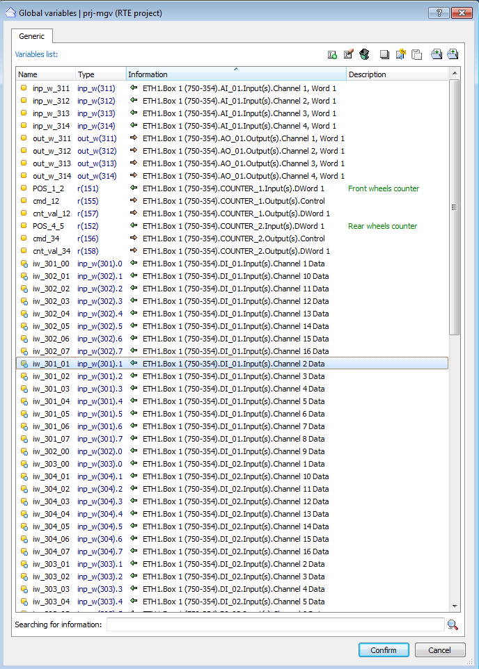
Global variable example

In this configuration we will assign manually IO addresses. We have one 16 digital input Wago module and one 16 digital output wago module. Even if each module is 16 bits, wago map each 8 bit on a word. So will have one 2 words for each module. As the animation, we assign the first 8 inputs of the module the address 300 and the first 8 outputs the address 300. Then we proceed incrementally. So the first 16DI module will be mapped to inp_w(300) and inp_w(301).

2.6.3. CanOpen

2.6.4. Profibus