4. R3 demos
All demos: of this chapter can be found in one workspace and one project.
4.1. Demo 1: Analog input
Le’t connect an analog temperature sensor to the analog module of Pheonix. Check RDE chapter for information about how to configure IOs.
The temperature sensor have linear relationship between the tension (V) and the temperature. The analog input have an internal 16 bit ADC (Analog to Digital Converter). The data type of the converted value is 16 bit (15bit + sign) Tension value is mapped from [0V;10V] to [0,30000]. Usually the max value 7FFF is more than 10V.
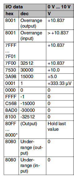
From datasheet of Pheonix AI module
The linear relationship between the signal and its phycical value is represented as:
\(m = \frac{(y_1 - y_0)}{(x_1 - x_0)}\)
\(y = m (x-x_0) + y_0\)
In our case the y will be the temperature and the x will be the digitalized value. To build a linear relationship we need two point \((x_0, y_0)\) and \((x_1, y_1)\). From the datasheet of the temperatura sensor we obtain the curve of the sensor.
- Let’s suppose that:
- 0V (AI=0) is \(0^\circ C\)
- 10V (AI=30000) is \(100^\circ C\)
The following is the code implemennted in R3:
$TASK 1

; Analog sensor connected to first analog channel of pheonix module
LIT temperaturaAI inp_w(36)	; Temperatura analog input

; temperature values are saved in non volatile real regisers
LIT temp0		nvrr(1)	; temperature
LIT temp1		nvrr(2)	; temperature
; scaling values. saved in non volatile integer registers
LIT temp0_ai	nvr(3)	; analog value corresponding to temp0 degree
LIT temp1_ai	nvr(4)	; analog value corresponding to temp1 degree

temp0 = 0.0
temp1=100.0

temp0_ai = 0
temp1_ai = 30000

real temperature = 0.0

__main_loop__

	; scaling equation, linear relationship between temperature and analog input
	; consult the datasheet of the analog module
		; 0V --> 0x00 (0)
		; 10V --> 0x7530 (30000)

	; Temperatura sensor
		; Range -45degree (1V) ~ 125 degree (10V)

	temperature = ((temp1-temp0) / (temp1_ai - temp0_ai) ) * (temperaturaAI - temp0_ai) + temp0

	; short task, we add a waiting instruction
	dwell(0.2)	; wait for 0.2 seconds
end_main_loop
4.2. Demo 2 : Using functions
In this section will show how to use functions. We will modify the temperature example, we create TASK2. First we create a function that represent a linear relationship between two variables linearmap(). Then we will call it in the main loop. In this example we will map the analog input into a register in order to be able to simulate it, as we don’t have the phycial sensor.
Note
remmeber to execute task2 form task1, by adding the instruction mt_en(2)
Note
We can force the value of inp_w in order to debug the program.
The following is the code implemennted in R3:
$TASK 2

; Analog sensor connected to first analog channel of pheonix module
LIT temperatureAI r(1)	; Temperatura analog input

; temperature values are saved in non volatile real regisers
LIT temp0		nvrr(1)	; temperature
LIT temp1		nvrr(2)	; temperature
; scaling values. saved in non volatile integer registers
LIT temp0_ai	nvr(3)	; analog value corresponding to temp0 degree
LIT temp1_ai	nvr(4)	; analog value corresponding to temp1 degree

temp0 = 0.0
temp1=100.0

temp0_ai = 0
temp1_ai = 30000

LIT temperature rr(1)


__main_loop__

	temperature = maplinear(temperatureAI, temp0_ai, temp0, temp1_ai, temp1)
	dwell(0.2)
end_main_loop

function real maplinear(int x, int x0, real y0, int x1, real y1)
	real m = (y1-y0)/(x1-x0)
	return m*(x - x0) + y0
end_fun
4.3. Demo 3 : Cylinder
In this demo we will illustrate the use of functions, and include files.
Remember that the code of included files, at compilation time are merged with the main file. It means the keyword $include filename.i3 is replaced by its content.
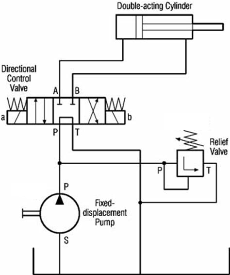
Hydraulic double acting cyclinder, 3 state electrovalve