1. Basics
1.1. RTE scheduler
RTE is a realtime preemtive operating system. The principles of RTE are quite simple. In a one core CPU, an operating system give the illusion to the user that it is executing programs, tasks or processes in parallel (in the same time). Even on a multicore computer, we have this illusion. Supposed our machine have a 4 core cpu, and we are using a webbrowser, a keyboard, a mouse, music player, a word processor, mail client, the OS is executing processes that the user ignore, etc. at the same time, 4 core are not enough to do the job.
Simply RTE allow execution of one motion task called RULE and 8 general purpose tasks. The rule have high priority, and it is a periodic task, that execute always at predefined time si, sampling interval. And tasks are executed in time sharing, for example 10 instruction from task1, then 10 from task2, and so on until task 8, then back agian to the following 10 instructions of task 1 and so on. This inifinite loop or iteration is interrpted at fixed time si by RTE in order to execute the RULE.
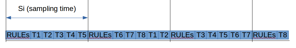
RTE scheduler. The execution of task depend on the sampling time. But RULEs are always executed periodically with a period equal to si`.
Note
The sampling time can be read from the predefined variable si. The period frequency can be set in RTE configuration.
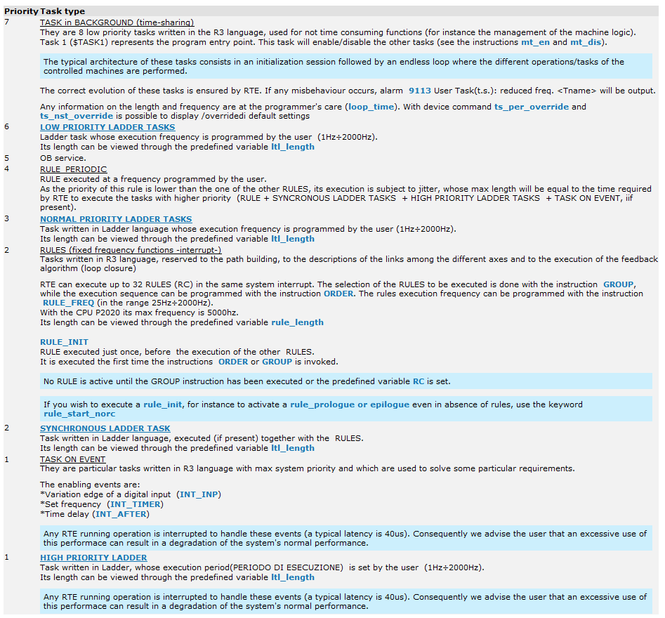
RULEs are a more complex concept. There are more then one rule, in RTE they are all executed together in sequence in the same sampling time. If RTE can’t execute them in one period, may be there are a lot of instruction and si is too short e.g. 0.2ms, RTE give an alarm and you have to increase si. Typical value si = 5ms on RP1.
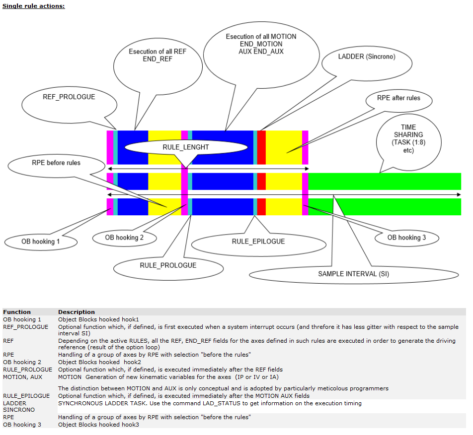
RTE can execute until 32 RULEs plus other 2 special ones called RULE_PROLOGUE and RULE_EPILOGUE. The sequence can be assinged in R3 program. Toegether with RULEs RTE execute other compenents. But for our purpose, we care only about RULEs.
You can immagine RULEs as different functions that RTE call in the sequence that you tell him. There is only one R3 program with the keyword $RULES where rules and other helper funtions are written.
Note
The rule file can have up to 1000 rules, but RTE can execute maximum 32 of them in the same sampling time.
Complete overview on RTE multitasking:
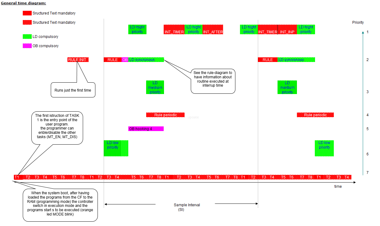
RTE multitasking
Priority
Rule execution
In this chapter we will create a simple demo in order to show how we can configure an axis (drive + motor) and simulate it.
1.2. Axis configuration
We will create three projects in one workspace, in order to illustrate different axis configurations:
- Ethercat
- CanOpen
- Analog reference
Each project reside in one folder in the workspace.
Multiproject workspace
Every axis have a unique name and a unique index, that can be used in R3 programs.
1.2.1. Analog reference
Let’s suppose we have a motor drive with analog reference speed control, and and feedback position.
Analog speed reference
We configure 2 axis, The first axis speed refrence is assigned to a volatile real register rr(1) and the feedback position to rr(11).
Note that we check emulated field in order to be able to emulate the drives. With a real drive, this field should be clear.
1.2.2. Ethercat
When controlling a drive via a bus, e.g. Ethercat, profinet, etc. we use PDO to control the drive.
- Important input words via bus:
- Status word : A mask that contain the status of the drive e.g. running, alarm, etc.
- Actual position or Actual speed
Importnat output words:
- Control word : A mask with command to the drive e.g. enable, run, etc.
- target position or target speed.
The role of each bit in the status and control words depend on the drive configuration.
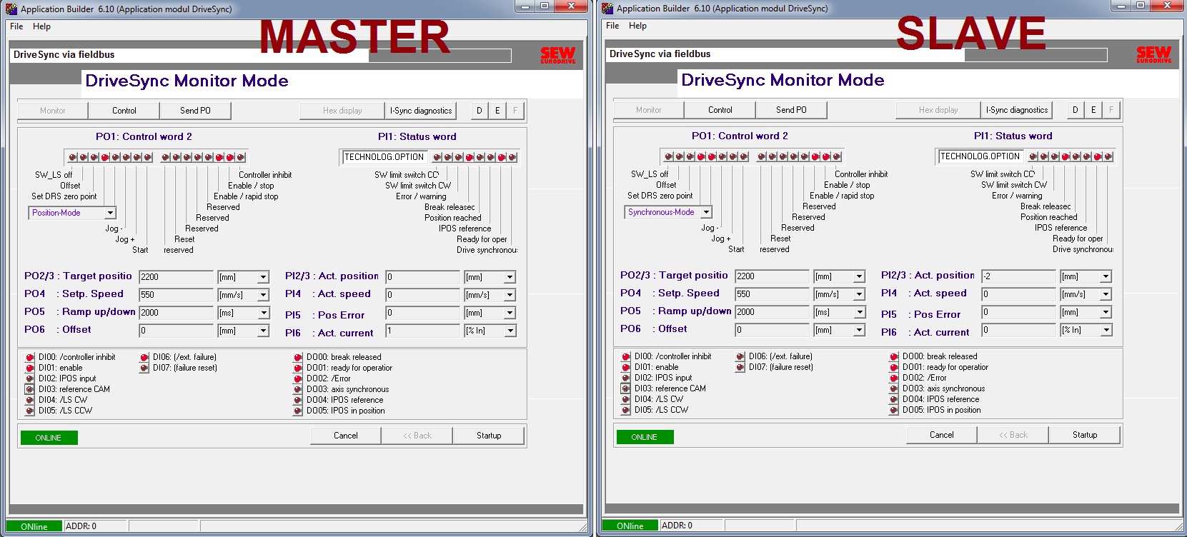
SEW Status and control word example of 2 different axis configuration.
1.2.2.1. Robox drive: IMD
Robox Integrated Drive
Robox IMD20: Ethercat
In order to congirure Robox IMD drives, you can use the predefined example.
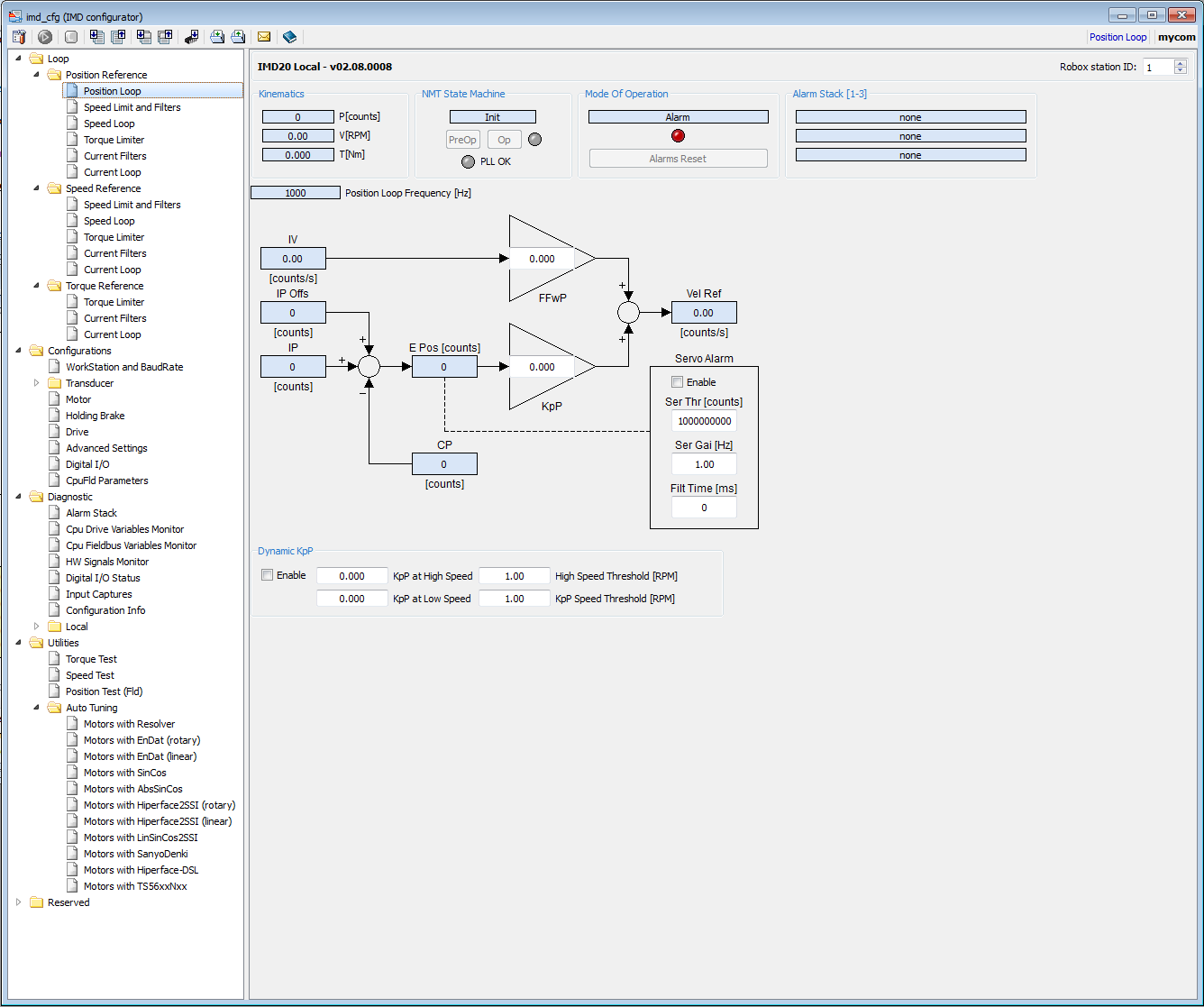
Robox IMD20: Configurator
1.2.3. CanOpen
1.3. Powerset
We can imagine the powerset as a logical power, for safety purpose, of a set of drives. For example we are controlling a 6-axis anthropomorphic robot and a 3-axis cartesian robot. We can create 2 power sets to group the 6 axis of the first and another one to group the 3-axis of the second one. Of course we can create 9 powersets, one for each axis. Suppose that the 3-axis robot have a problem and need to stop, it is logical to stop all 3 axis.
Powerset
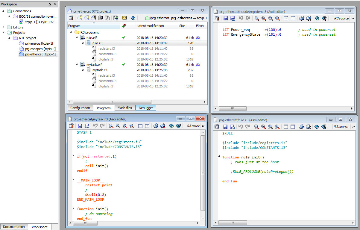
In the powerset configuration we select the axis, which power is handedled by the powerset the we call ps. If axis are controlled via a bus e.g. Canopen over Ethercat, as feedback we choose CANopen(CAN402). Usually even if drives use fieldbus, saftey circuit still exist. Suppose we have an emergency circuit, that is connected to the controller which state can be read in r(101).0. In the powerset feedback we add also that register.
If the feedback signals are HIGH, the powerset can be energized by the signal that set in the tab requests POWR_RQ, power request. In our case, we choose r(100).0. Imagine the powerset as a safety realy, if safety condition are met feedback = true, the relay contacts can be closed under a request from POWR_RQ.
You can find a ready to use graphic panel to monitor the powerset. Later we will see how to use it.
To enable power of different axis, a chain of power in the power set have to be enabled, like a safety chain. There are some predefined variables and funtions that manage axis power. We will some of them in order of chain hierarchy, top-down view:
power_allowed: Flag that enables all the PowerSetsps_power_enable(POWER_SET ps, I32 flag): Enables the PowerSetpsif flag == 1.ps_channel_enable(POWER_SET ps, I32 enableMask): Enables the drives of the PowerSetps, where the drive relativ bit is 1. e.g.enableMask=0x05only axis(1) and axis(3) are enabled.
POWER_SET is a STRUCT to define a powerset. for example the field eba is a flag related to system alram, if it is true, it means there are no alram that forbide the power to be energized.
Consult the documentation in RDE RTE firmware –> power handling and related arguments where you can find also a state machine of power handling.
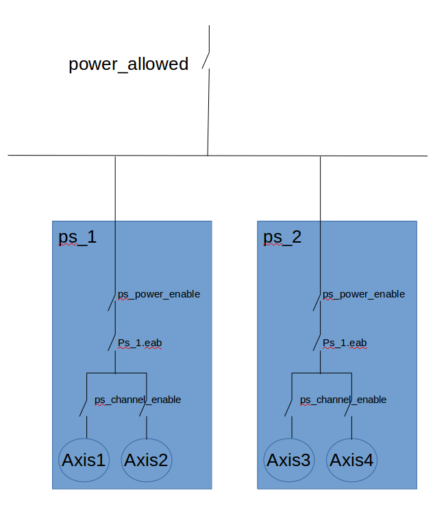
Powerset enabling chain
1.4. RULEs
We prepare the base project, that let us to complie with errors. Remember that in order to compile a task, at least one instrution should be present.
Powerset enabling chain
Rules are similar to function that handle motion instruction. We can use different rules to manage an axis state machine, or we can use one rule where we can write the state machine directly. One RULE can handle up to 32 axis. In the rule body, the required axis are selected. The main strucure of a rule is:
RULE number
  axes n[,n,n,...,n]

  ref
    ; optional block of instructions containing the position loop closure algorithm.
  end_ref

  motion
       if(first_time())
          ; solo la prima volta
       endif
       ; block of instruction containing the algorithms to build the ideal trajectory
  end_motion

  aux
    ; optional block containing auxiliary instructions
  end_aux

END_RULE
If the rule is active, it is executed one time every period of the RULEs execution, one time every si. The ref and aux blocks are optional. So for now we don’t discuss them. Remember the rule number is unique.
Let’s write a code to move an axis in jog mode.
rule R_JOG
      ; axis 1
      axes(1)

      motion
      jog = bJogPos - bJogNeg ;
    ; MVA_JOG2(I32 ax, I32 direct, REAl speed, REAL accel, REAL decel)
      res = MVA_JOG2(axis_x, jog,      10,               100,        100,  1, 1, 0)
      end_motion

end_rule
Motion instruction can be found in R3 documentation. Check also the predefined variables in R3, related to motion control. This rule when active, handle the motion of axis 1 only, axis(1). When jog = 0 the axis doesn’t move, when jog=1 it move in positive direction when it is jog=-1 it move in negative direction.
We can use different RULEs to assign different behavior to the axis. For example one Rule for jog motion, one for homing, one for positioning, etc.
We have two special rules, RULE_PROLOGUE and RULE_EPILOGUE. RULE_PROLOGUE is executed by RTE before the motion block of all active rules and RULE_EPILOGUE is executed after them.
rule_init() is a special function executed by RTE at the first execution to initialize the rule, e.g assign RULE_PROLOGUE.
function rule_init()
  ; if needed we enable the execution of the
  ; rule_prologue and rule_epilogue in the initialization rule
  rule_prologue(func_prologue)
  rule_epilogue (func_epilogue)
  ; do something
end_fun

function func_prologue
  ; do something
end_fun

function func_epilogue
  ; do something
end_fun
First let’s define some rule to manage an axis, then define a state machine to assign rules depending on the requirments. We begin to define some constants, to assign a name to rules:
LIT R_POWER_MISSING   1
LIT R_FAST_STOP       2

LIT R_IDLE            3
LIT R_HOMING          4
LIT R_JOG             5
LIT R_POSITIONING     6
LIT R_AUTO            7
We will present some of the rules code, the complete code is found in the attached demo:.
rule R_POWER_MISSING
      axes(1,2) ; only axis 1 and 2 is managed by this rule
      motion
         res = mva_open_loop(ax_x)
     res = mva_open_loop(ax_y)
      end_motion
end_rule
We can write also the axis name in the function axis()
axis(axis_x, axis_y)
The motion funtion mva_open_loop(axis_number), assign the actual position to the ideal position ip(axis_number) = cp (axis_number). This can be done when power is missing, to avoid any gap between the ideal position and the acual one, when the axis is powered and avoid any sudden motion.
Let’s suppose we want to stop the axis in a controlled way when emergency circuit is opened, or to some grave error happen. So we have to ramp down the motion of the axis, ramp down the speed to zero, quickly and avoid sudden stop.
rule R_FAST_STOP
      axes(axis_x, axis_y)
      motion
              iv(axis_x) = ramp(iv(axis_x), 0, max_acc(1)) ; ramp down ideal speed to 0
    iv(axis_y) = ramp(iv(axis_y), 0, max_acc(1))
      end_motion
end_rule
Notice that we write only the ideal velocity or ideal position. Here we supposed that the drive close the velocity loop, and the deafult control loop of RTE is executed. More about this topic when we examine the ref block.
Now we write the code of the posiiotn rule. The rule have to move the axis to a defined poistion:
rule R_POSITIONING
  axes(axis_x)
  motion
    ip(axis_x) = mv_to (MovResult, 1, lTarget, lSpeed, lAcc)
    if ( rise(MovResult = M_REACHED and similar(ip(1),lTarget,1) ) )
      ; do something
    end_if
  end_motion
end_rule
We already see how we can defined RULEs to do different things with axis, it is a simple concept. It is like writing functions to divide the tasks to do in a machine. We see also some motion instructions and how to used predefined variables related to motion control.
More motion control instructions can be found in the documention of R3 language.
1.5. Standard position loop algorithm
A rule contain the ref block that is optional, where control algorithms can be implemented.
If the block is omitted, RTE will execute its standard, preimplemented control loop. In this case the controller will close the position loop, give a speed reference to the drive and the drive will close the speed loop and eventually other internal loops.
; n is the axis index
epos(n) = p_ip(n,ipp_idx) – cp(n)
sref(n) = epos(n) * pro_gai(n) + kff(n) * iv(n)
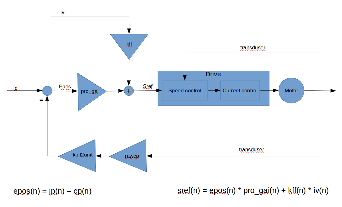
RTE standard closure of the proportional position loop with speed feed forward
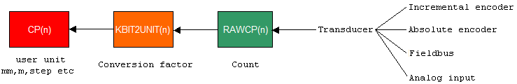
Transduser count to physical unit convertion
1.6. RULEs execution
In our example we will enable one rule at one time. But in a multiaxis more complex machine we need to enable a group of axis, and maybe different rules at the same time. There are instruction to assign to RTE the execution order of the enabled order, in every sampling time.
The predefined variable rule_length give the execution time of what we call RULE. Remember that we don’t mean a single rule, but the set of funtions, OB, etc. related to motion. So the time return by thi variable is the execution, let’s say of everything exluding normal tasks. rule_length can’t be bigger then si. Remember that in one period, si, RULES and some slices of tasks have to be executed. The rule frequency is set by the function rule_freq (I32 freq) or in RTE project configuration. The variable si is read-only. If the execution time is not enough, the rule frequency have to be increased.
Rules can be enabled when need, from a taks or from another rules. We can enable Rules, using different R3 functions. First we need to declare a variable of type STRU_GROR it is a STRUC which contain an array of I32 idx[32]. This strucure is used with the instructions group(STRU_GROR rulegroup) or order(STRU_GROR rulegroup), and the meaning of each element depend on the instruction used.
RTE rule executer use a predefined variable rc(n), which is an array of 32 elements. The value of rc(n) is a rule number. The standard order of rule execution is from index 1 until the last one. The order of execution can be changed using the instrction order().
Let’s make some example. First let’s execute the rules in rc as are predefined in RTE, begining from the first one, so we don’t use the instruction order().
In the follwing example, we define the strucure rule_group, then we assign the number of rule to be activated. The index of idx is the order of execution of the rules, that correspend to the index of rc.
STRU_GROR rule_group

rule_group.idx[1] = 5 ; rule number , rc(1)=5
rule_group.idx[2] = 2 ; rule number
rule_group.idx[3] = 1 ; rule number
rule_group.idx[4] = 100 ; rule number

group(rule_group)
Now let’ change the execution order of the rules. Let’ execute in sequence rc(4), rc(1), rc (3) then rc(2). The execution order will be RULE 100, RULE 5, RULE 1 then RULE 2.
STRU_GROR rule_order
STRU_GROR rule_group

rule_order.idx[1] = 4 ; 4 is rc index
rule_order.idx[2] = 1 ; rc index
rule_order.idx[3] = 3 ; rc index
rule_order.idx[4] = 2 ; rc index

group(rule_group)

rule_group.idx[1] = 5 ; 5 is rule number , 1 is rc index. rc(1)=5
rule_group.idx[2] = 2 ; rule number
rule_group.idx[3] = 1 ; rule number
rule_group.idx[4] = 100 ; rule number

group(rule_group)
In summary, with the instruction group we assing rules to rc, e.g. rule_group.idx[6] = 23 equivalent ot rc(6) = 23. And with the instruction order we change the order of exection of the rc, in other word we remap the indexes of rc.
We can assign -1 to rule_order.idx[n], in order to telle the executer that n-1 is the last rc to be executed.
STRU_GROR rule_order
STRU_GROR rule_group

rule_order.idx[1] = 4 ; 4 is rc index
rule_order.idx[2] = 1 ; rc index
rule_order.idx[3] = 3 ; rc index
rule_order.idx[4] = -1 ;
Finally we assign rules to the ruel executer using directly the variable rc.
rc(1) = 2
rc(2) = 35
rc(3) = 9
rc(4) = 1
rc(5) = 5
rc(6) = 7
Remember that task execution can interrupted, in order to execute another task or rule. This mean that, if the task is interrupted by the rules before the controller execute rc(4), only rc(1), rc(2), rc(3) will be assinged to the rule executor. And the others will be assigned in the follwong sampling time.
For this reason is better to use the instruction group, in this way all rules defined in STRU_GROR will executed.
1.7. Power
In another chapter we will examine a complete example, where we implement a state machine that enable rules depending on the machine requirment. In this section we will see some R3 instructions in order to deal with power handling.
In the initialization function, in TASK1, we need to enable the powerset and single axis:
ps_power_enable(ps,true)  ; enable powerset ps

; I32 ps_channel_enable (POWER_SET psname, I32 enableMask)
ps_channel_enable(ps,0x3) ; enable axis 1 and 2 in the powerset ps
We can invetigate the status of the powerset, using the instruction I32 ps_status (POWER_SET psname) that return:
0x00000001 (B0) at least 1 drive in fault
0x00000002 (B1) Powered
0x00000004 (B2) at least 1 drive enabled
0x00000008 (B3) all the powerSet drives are enabled
0x00000010 (B4) delayed (if required) state of the feedback
0x00000020 (B5) reserved
0x00000040 (B6) counting running in case of delay because of axis alarm causing the power drop (power_off_delay_on_alarm)
0x00000080 (B7) counting running in case of delay because of feedback lack (power_off_delay_on_no_feedback)
0x00000100 (B8) actual feedback state (not delayed)
0x00000200 (B9) the feedbacks for all the drives are present
0x00000400 (B10) the feedbacks of all the drives for which the enable command has been activated, are present (instruction ps_channel_enable)
B11-B32 Reserved
For example we want to see
 if ( ps_status(ps) r_and 0x8)
  ; all the powerSet drives are enabled
 end_if

systemPowered = ((ps_status(ps) r_and 0x12) = 0x12) ; x012= 0x10 OR 0x02

powerGoingDown = (ps_status(ps) r_and 0xC0) ; C0 = 0x40 OR 0x80
1.8. Summary
TODO